


![Request for Information – Potential [Placeholder for Prize]](https://assets.science.nasa.gov/dynamicimage/assets/science/psd/solar/2023/09/s/solarsystem_0.jpg?w=1024)


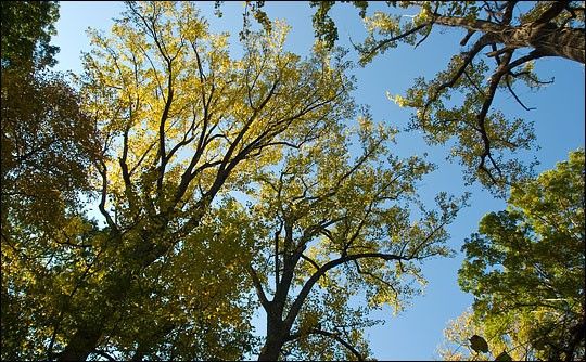
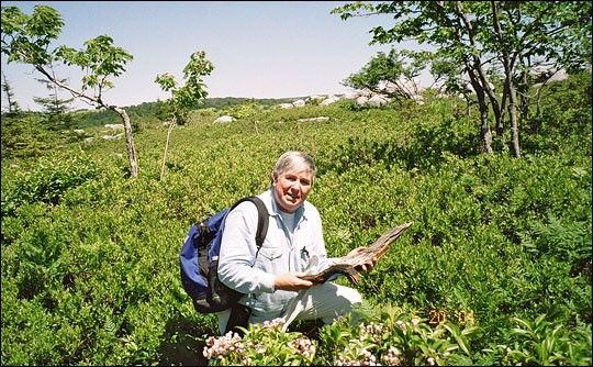
“Wow, that’s a beautiful tree.” Louis Steyaert has his head tipped back to make out the outline of the autumn leaves that cling to the uppermost branches of the giant tulip poplar. Tens of meters overhead, the trunk splits, the two branches racing towards a clear November sky. “How old do you think it is?” Steyaert asks, turning to his colleague, forest ecologist Robert Knox, who is respectfully considering the tree. Leaves crunch as Knox steps forward and embraces the mossy bark, his arms spanning perhaps two-thirds of the massive trunk.
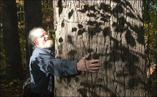
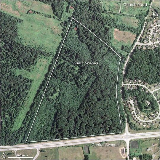
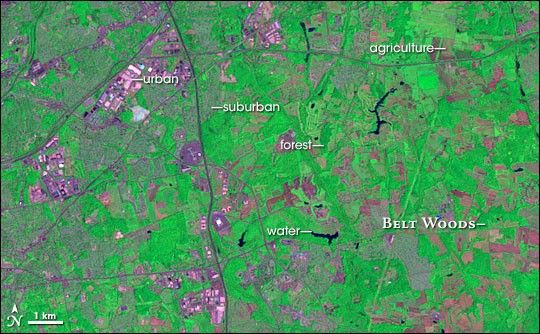
“At least pre-settlement,” he says, stepping back. Several of these giants are scattered across the sloped, 109-acre Old Belt Woods, which contains one of the last remaining tracts of virgin forest in the eastern United States. Steyaert and Knox have taken me to this tiny forest enclave to give me a firsthand experience of the kind of mature forest that once covered nearly the entire United States east of the Mississippi.
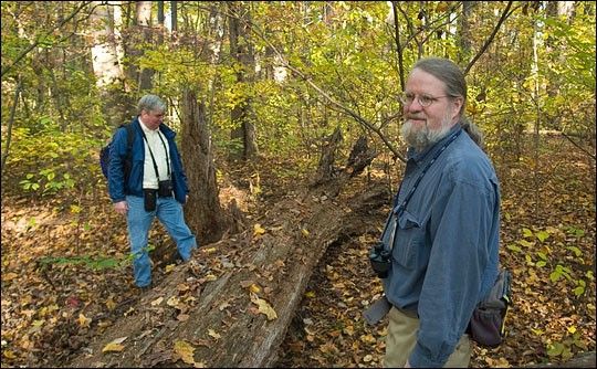
“This is one typical sign of old growth,” says Steyaert, pointing to a large, centuries-old tree lying across the forest floor. A pit sinks behind the tree’s upturned roots. In forests regrowing on land that was once cleared and plowed, the pits left by falling trees are smoothed over. A truly ancient forest is crater-marked. In a nearby gap left by another fallen giant, a cluster of young tulip poplars compete to fill the space. The massive trees, fallen logs, gaps, and seedlings make the forest uneven; this unevenness is a hallmark of an old, multi-generational forest.
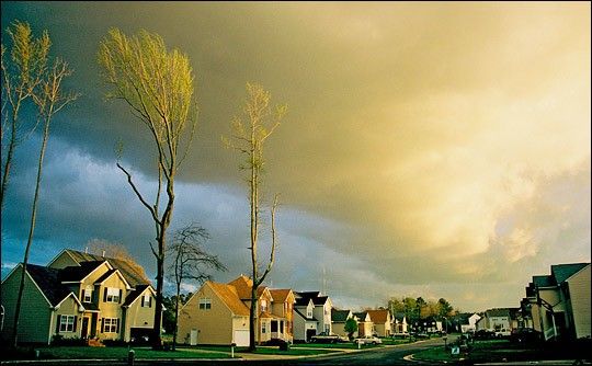
Is this what North America looked like when John Smith explored it? For Steyaert and Knox, the question is more than idle speculation. Plants interact with the atmosphere to influence local weather and climate. As the landscape changed from forest like Old Belt Woods to the suburban environment surrounding it today, did the weather change as well? Could future changes intensify or lessen global warming by tweaking local weather patterns?
As we stand in the woods talking, the wind rushes through the uppermost branches, snapping the leaves that remain on the trees. Standing in the calm below, I can easily see how such large trees hold sway with the wind, but climate models need a different kind of description to reach the same conclusion. They need numbers that describe the shape, height, and color of the tree-tops and the density of the leaves because these are among the elements that talk to the atmosphere.
Describing landscape changes in the eastern United States since colonization began and translating those descriptions into numbers models can use was the Herculean five-year task that the pair of scientists standing in Old Belt Woods with me that fall day had just completed. Using everything from observations recorded by naturalists and foresters throughout the past 150 years to data from Earth-orbiting satellites, Steyaert and Knox created a series of maps that reconstruct the landscape as it would have appeared in 1650, 1850, 1920, and 1992. These maps provide the hard numbers that climate modelers need to determine what effect landscape changes might have had on the weather in the eastern United States.
What is a Model Forest?
To find out how a forest or a field of wheat influences weather or climate, modelers simulate the intricate interactions between land and sky. The goal, says NASA modeler Lahouari Bounoua, is to first understand how a single molecule of carbon dioxide is pulled into a leaf in exchange for oxygen and water vapor, and then to scale that interaction up until the model describes the impact of all Earth’s vegetation on its climate. To do this, modelers need to know specific biological and physical characteristics—modelers call them “biophysical parameters”—of the landscape, everything from leaf density, to root depth, to canopy height. Biophysical parameters change from landscape to landscape.
Steyaert, a climate and atmospheric scientist visiting NASA Goddard Space Flight Center from the U.S. Geological Survey, has spent much of the past decade mapping regional land cover and biophysical parameters for regional climate models. He has scoured books and other scientific literature to understand how the landscape of the past looked, and he reconstructed historical landscapes in the eastern United States for four snapshots in time: pre-colonial, 1850, 1920, and 1992. Then he asked NASA ecologist Robert Knox to help him develop the next generation of landscape data that would include not only landscape categories—like forest or farmland—but also historical biophysical parameters, the “real numbers” that regional climate models depend on.
Having worked with climate modelers on a previous forest-mapping project and having spent a lifetime observing forests first hand, Knox knew that to understand the impact of land cover change on climate, you had to understand in detail how land use changes the biophysical nature of the forest: the way it disturbs the wind, reflects light, evaporates water, or cools the ground. All these changes, Knox understood, had to be represented by different numbers in climate models.
The Ancient Forest: 1650
When Steyaert asked him about mapping the forest of 1650—after native land use had declined in the wake of disease brought by early Europeans but before colonial farms took off—Knox already had firm ideas about where to start: the scientific studies of August Wilhelm Küchler. A plant geographer in the mid-1900s, Küchler had spent his career painstakingly mapping the distribution of plants across the United States. Küchler considered soil types and climate to determine what kind of vegetation would have been growing in the United States if the land had been left undisturbed by human activities.
“Other people had used Küchler data,” says Knox, “but my opinion is that there is a terminology barrier.” Modelers took Küchler’s “evergreen forest” category, for example, and applied the same biophysical values to all evergreen forests, whether they were in the White Mountains of New Hampshire, where the average tree height was 10-20 meters, or the Deep South, where a 50-year-old loblolly pine can reach 30 meters. “Even if you treat all conifer needles the same,” explains Knox, “just the architecture of the forest would change how it interacts with the atmosphere.”
What modelers had previously overlooked was the manual that went along with Küchler’s potential natural vegetation map. The manual plus Küchler’s related scientific publications detail what kinds of plants would grow in each specific vegetation type, or land cover class, with a description of the land-cover characteristics. Küchler describes the oak-pine forest of New England, for example, as a “medium tall forest of broadleaf deciduous and needle leaf evergreen trees. In places the forest is low, even shrubby.” Knox realized that these descriptions—dense, sparse, scattered, medium tall, shrubby—contained a wealth of information that could be used to estimate biophysical parameters.
As the first step, Knox translated Küchler’s vegetation classes into a set of consistent land cover classes that represented the foundation for the 1650 land cover and a suitable framework for subsequent land cover changes. For his part, Steyaert realized that while Küchler’s descriptions were excellent, they were based on observations made between the 1930s and the 1960s, after many changes to the native landscape had already taken place. Using older descriptions gleaned from hours in the library, Steyaert identified limitations in the Küchler’s vegetation classes and defined additional land cover classes to account for some of the well-documented land use changes after 1650.
The next task, then, was to translate Küchler’s modified land cover classes into estimated biophysical parameters, the “real numbers” that determined the interactions between the land and the atmosphere. Modelers need to know, for example, exactly how much sunlight the land reflects compared to how much it absorbs, a value called albedo. Light-colored land cover, such as snow or pale sand, has a high albedo, or reflects most of the sunlight that hits it. A dark pine forest, on the other hand, absorbs more of the Sun’s energy and so has a low albedo. Steyaert and Knox compared Küchler’s vegetation types and current vegetation with modern measurements of albedo recorded both in field studies and by satellite instruments such as NASA’s Moderate Resolution Imaging Spectroradiometer (MODIS). Field measurements might indicate that a low, shrubby forest that contained both evergreen and broadleaf deciduous trees like oak had an albedo of 0.13, and so, Steyaert and Knox estimated that those places that Küchler designated as being covered by low, shrubby mixed forests had an albedo of 0.13.
Over the next three years, Knox and Steyaert would come up with biophysical parameters for all the land cover classes they would need to classify U.S. vegetation during each of the four time periods they planned to map. They estimated values for vegetation characteristics such as leaf area, the ratio between the number of leaves that cover an area and the ground area; deciduousness, what proportion of the leaves disappear during cold winter months; canopy height, the height of the tallest layer of plants in a forest or grassland; and surface roughness, the amount of turbulence the plants create as wind blows around them.
But how had those parameters changed as the United States was settled? To determine what had changed, Steyaert and Knox turned to the first quantitative record of land cover change in the United States: the 1850 census.
Fields and Forests: 1850
Sandwiched between “Professions, Occupations, and Trades of the Male Population” and an accounting of livestock and produce during the year ending June 1, 1850, the 1850 agricultural census estimates the acres of “improved” or “unimproved” farmland per county within each state. The scientists classified the rest of the estimated county area as “non-farmland,” but these categories left a lot room for interpretation.
To figure out what farmland, unimproved farmland, and non-farmland looked like in each county, Steyaert consulted books and other documents that included historical references dating back 100 years or more in some cases. “Improved farmland basically meant that the land was cleared and used for cultivated crops, pasture, or grassland for hay,” says Steyaert. Farms in highland areas like the Appalachian Mountains would have been different from farms in lowland areas because of differences in elevation, slope, soils, and climate.
“Unimproved farmland” could have been an undeveloped frontier claim with the old-growth forest still intact, or a wooded area being used for timber, fuel, or livestock grazing. “Non-farmland” could have meant anything from a village to undisturbed wilderness. How could they decide which scenario was more likely? From the historical information, it became clear that the more populated a county was, the more likely it was that “unimproved farmland” meant a disturbed woodlot and not old-growth forest, and the more likely it was that “non-farmland” meant a village or city and not forest or other natural vegetation.
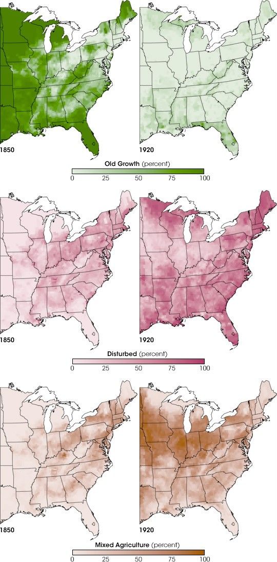
They decided the best way to map out the fraction of changed and unchanged land in 1850 was to estimate the percent of a county’s land that fell into each of four “land use intensity” categories: highland agriculture and lowland agriculture (based on “farmland” estimates from the census and topographic data), and forest-village disturbance and old-growth forest (based on population density data). These maps revealed how much impact people were having on the landscape in each county and how much area of the pre-colonization land cover classes remained. From there, the scientists could calculate how the climate-relevant characteristics—the biophysical parameters like albedo and surface roughness—had changed as well.
The resulting maps showed drastic changes in the landscape between 1650 and 1850. Most of the coastal forest had disappeared. A line of virgin forest traced the peaks of the Appalachian Mountains, and much of the southern forest remained intact. The Upper Midwest was starting its transformation to farm land, though the western frontier, west of the Mississippi, remained relatively untouched. All would be entirely transformed in the era that followed the U.S. Civil War, changes that became evident in the agricultural census of 1920.
Cities, Farms, and Forests: 1920
By 1920, people were intensively using most of the land in the eastern United States. The age of mechanized agriculture had dawned, and farms were supporting a much higher population base. Although much of the old-growth forest had given way to crops and pastures or villages and cities, forests were re-growing in farm woodlots and previously logged areas, and semi-natural vegetation was beginning to reclaim abandoned farms. This change brought new challenges for Steyaert and Knox. What did the 1920 vegetation look like for each of these land cover types?
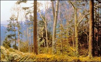
Undisturbed forests, such as those that grew in 1700, contain trees of varying size and age. Tall trees block sunlight so other plants don't grow well near them. This creates an open forest floor with gaps between the trees.
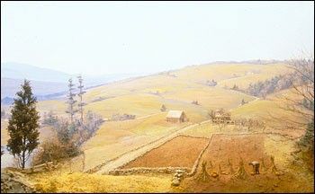
Farms present an entirely different profile to the atmosphere. Smooth fields offer little resistance to the wind; lighter-colored crops reflect more sunlight; and with fewer leaves than a forest canopy, crops respire less water and soak up less light in photosynthesis. These differences can change local weather.
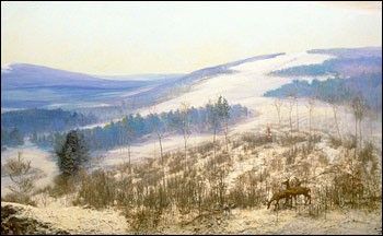
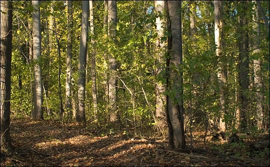
Trees growing over abandoned fields are packed closely together. The trees all have similar heights, and the land beneath them is still smooth and even after cultivation. The even canopy means that a regrowing forest interacts with the wind differently than an old-growth forest. (Harvard Forest Diorama Photographs © 2002 Fisher Museum, Harvard Forest, Petersham MA. Photography by John Green.)
“We used a wide variety of sources in the recent and historical literature to reconstruct the 1920 land cover conditions,” says Steyaert. “I visited the National Agricultural Library and read the U.S. Department of Agriculture Yearbooks from 1921 through 1925 and other really early books. The libraries at the University of Maryland, NASA Goddard, and the U.S. Geological Survey were also gold mines,” Steyaert recalls. He found regional information on the estimated acreage of regrowing forest and remaining virgin forest with commercially useful timber, as well as many other maps of land use activities based on the 1920 census.
Using the census data for both population and farm area along with the other sources of information they resurrected from library archives, the pair developed land-use intensity maps and used them as a basis for mapping the fraction of each county that was lowland or highland agriculture, remnant old growth, and residential and urban areas.
Among the new challenges was figuring out how to describe what was happening on farm woodlots and non-farmland that didn’t seem to be either city or old-growth forest. Using census records, regional forest area estimates, and Küchler’s vegetation maps, they split the remaining non-farmland and the farm woodlots into two major components. The first was young, regenerating forest, and the second was “non-restocking land,” where the returning vegetation wasn’t the forest that had grown in the area before.
So what was growing in those areas that foresters called non-restocking? “In some cases,” says Steyaert, “the vegetation growing back after logging was like some kind of scrubby oak or pine.” In other locations, such as peat bogs, tree growth is naturally slow. “If the area is blanket peat lands,” says Knox, “and you take off the spruces that actually have had a long enough time to get big enough to be worth cutting, that would be non-restocking. A thirty-year-old spruce might be half a meter tall there.” Even 20 years after logging, the area would be ‘non-restocking’ in terms of commercially useful timber, even though mosses and shrubs would exist.
Grouping the logged, non-restocking forest with degraded farmland identified in the 1920 census, Steyaert and Knox derived a land cover class and biophysical parameters for “degraded land.” “We characterized degraded land as having sparse vegetation, scattered shrubs, scrub trees, and barren land with poor forest regeneration,” says Steyaert. Their analysis showed that by 1920, the original forest had all but disappeared, and virtually no part of the eastern United States remained unchanged at the 20-kilometer scale depicted in the maps.
Steyaert and Knox were ready to move to something closer to the present, and this time, they got a break.
The Forest Returns: 1992
“Compared to 1920, 1992 was pretty easy,” says Knox.
“We had images and land cover data from Landsat,” Steyaert explains.
Steyaert and Knox derived their land use intensity, modern-day land cover, and biophysical parameter maps in large part from analysis of the 1992 USGS National Land Cover Dataset, which is based on Landsat satellite data. Since 1972, a series of Landsat satellites have orbited Earth, giving a detailed picture of land cover by recording reflected light and energy and providing an actual measurement of some of the biophysical parameters. For Steyaert, seeing color images of Landsat data captured in 1992 was as easy as walking down the hall from his office at NASA Goddard Space Flight Center. Hanging on the wall was an 8-foot-by-12-foot mural of the United States made from hundreds of Landsat images. “I still go down there and spend time studying the landscape features, literally from coast to coast, comparing my mental and 35 millimeter pictures of places visited with Landsat, and thinking about changes since 1650.”
“Between 1920 and 1992, the forest regenerated,” says Steyaert. “But it’s not the same forest as in 1650. For example, the albedo maps show the relatively low albedos of the darker forest in 1650, higher albedo values with agriculture and landscape fragmentation in 1850, maximum albedos with the intensive land use of 1920, and then intermediate values of albedo in the areas of forest regrowth by 1992.” Canopy height and surface roughness changed, too, with maximum tree height in 1650, minimum heights in 1920, and partial recovery by 1992.
“Altered soil moisture levels in the early growing season as a result of the conversion of various types of wetlands to agriculture by artificial drainage systems represented another important land cover change over time of interest to modelers,” Steyaert adds, pointing out the former areas of seasonally wet prairies within the Upper Midwest and wetlands in the lower Mississippi River Valley. “By 1992, agriculture became much more regional, and much more mechanized and intensive, centered on the Corn Belt and the lower Mississippi River Valley. And of course, there’s been urban growth and fragmentation of the landscape.”
“I was somewhat surprised as the study unfolded by the degree to which vegetation in the eastern United States hasn’t recovered,” says Knox. “There is very little forest in the East left that is like the pre-settlement forest, and the degree to which that translated into biophysically important parameters was a surprise.”
A Change in the Weather?
If the biophysical parameters influencing the interactions between the atmosphere and the land changed so dramatically over the entire eastern half of the United States, how has the weather changed? This is the sort of question that can’t be answered without plotting the changes in a model, says NASA Earth system scientist Jim Collatz. “You could have more extreme climate events. You may have longer droughts or more thunderstorms or localized thunderstorms. You don’t know until you run a climate model.”
You need a model, says climate researcher Roger Pielke, Sr., a senior research scientist at the University of Colorado in Boulder, because the changes in the biophysical parameters have competing effects on the weather. “If you cut down a forest, you might make a surface that has a low albedo go to a higher albedo,” says Pielke. Since higher-albedo surfaces reflect more and absorb less of the Sun’s energy than low albedo surfaces, they tend to be cooler. “But then, you might have less water to transpire,” Pielke continues. Plants breathe out water, which cools the air. If the trees are gone, less water will enter the atmosphere, leading to warmer temperatures. Between the competing effects of a higher albedo and lower water content, “you still might have a higher temperature,” says Pielke.
“I think the bottom line is that our study area represents roughly half of the conterminous United States, and we can see that a lot of major changes have taken place since 1650,” says Steyaert. “The fundamental question is, given these historical land cover and land use changes and their effects on the biophysical parameters, what will the modeling experiments reveal about the consequences for land and atmosphere interactions?”
Pielke and his colleagues have already started to run Steyaert and Knox’s land cover and biophysical parameters data in a regional climate model. Preliminary results show temperature changes that vary by region. As experiments go forward, the weather-related consequences of past land use decisions will become clearer. In addition, we may learn something about how the land use decisions we make today will affect the weather tomorrow. Perhaps leaving or planting a swath of native forest such as Old Belt Woods within our cities or suburbs will be a part of moderating local weather and adapting to global warming.
References
- Braun, E.L. (1950). Deciduous Forests of Eastern North America, Philadelphia: Blakiston Company.
- DeBow, J.D.B. (1853). The Seventh Census of the United States: 1850. Washington, D.C.: Robert Armstrong: Public Printer. Reprinted in Historical Census Publications. United States Department of Agriculture. Accessed December 3, 2007.
- Denman, K.L., G. Brasseur, A. Chidthaisong, P. Ciais, P.M. Cox, R.E. Dickinson, D. Hauglustaine, C. Heinze, E. Holland, D. Jacob, U. Lohmann, S Ramachandran, P.L. da Silva Dias, S.C. Wofsy and X. Zhang. (2007). Couplings Between Changes in the Climate System and Biogeochemistry. In: Climate Change 2007: The Physical Science Basis. Contribution of Working Group I to the Fourth Assessment. Report of the Intergovernmental Panel on Climate Change [Solomon, S., D. Qin, M. Manning, Z. Chen, M. Marquis, K.B. Averyt, M.Tignor and H.L. Miller (eds.)]. Cambridge University Press, Cambridge, United Kingdom and New York, NY, USA.
- Küchler, A.W. (1964). Potential Natural Vegetation of the Conterminous United States. New York: American Geographical Society.
- Steyaert, L. T., and Knox, R.G. (2008, January 16). Reconstructed historical land cover and biophysical parameters for studies of land-atmosphere interactions within the eastern United States. Journal of Geophysical Research. 113, D02101, doi:10.1029/2006JD008277
- Williams, M. (1989). Americans and their Forests: A Historical Geography. Cambridge, New York, Melbourne, Madrid: Cambridge University Press.
NASA Earth Observatory story by Holli Riebeek; design by Robert Simmon