


WFI Reference Information
This page has the current version of Roman WFI Performance. This is v1.4, March 2026. [view version history]
Wide Field Instrument (WFI)
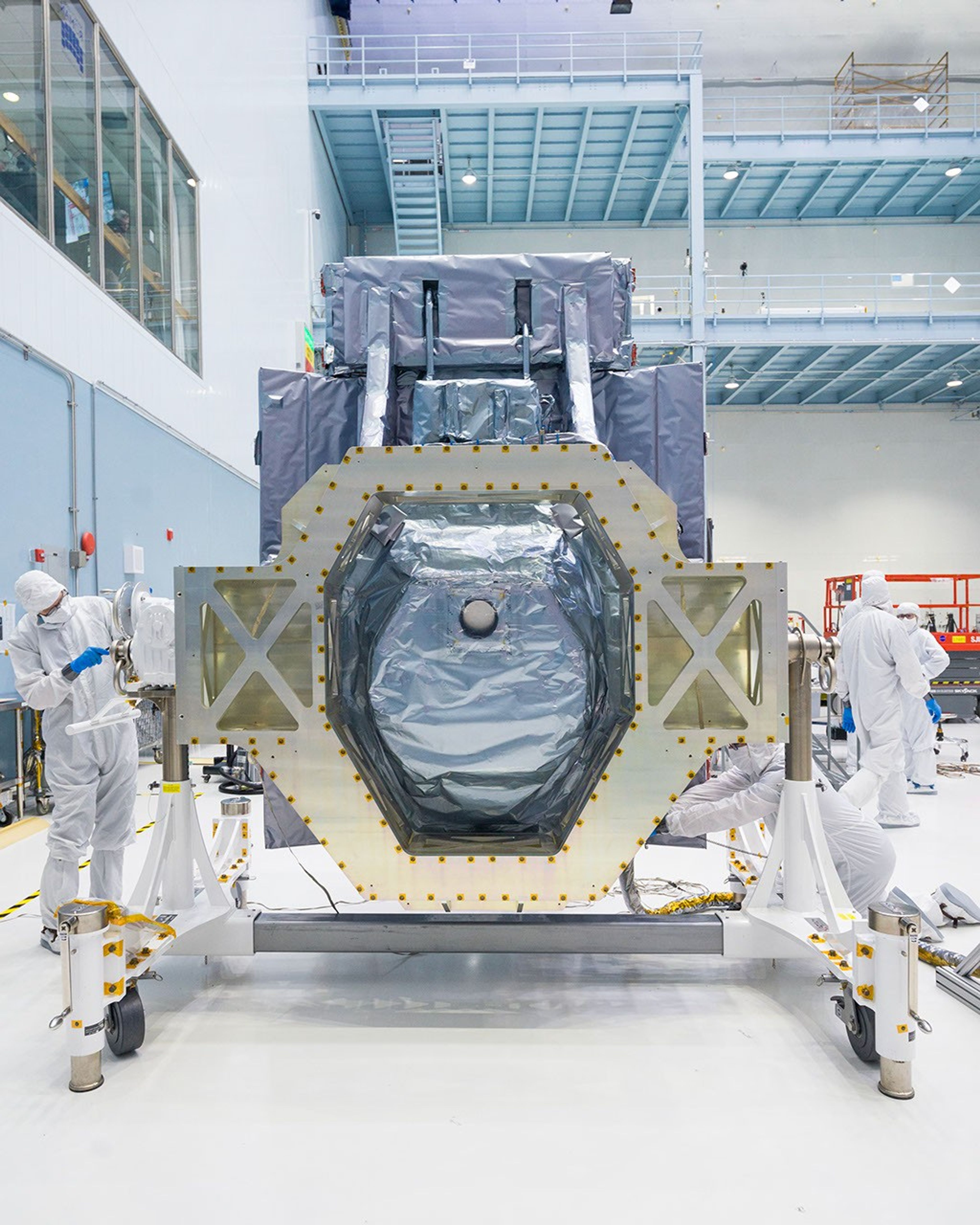
The Wide Field Instrument (WFI) is Roman’s primary science instrument and enables large scale surveys. The WFI is a 300-megapixel visible-to-NIR imaging camera and slitless spectrometer. In the full Roman Observatory, the WFI is composed of two major components: the Cold Sensing Module (CSM) and the Warm Electronics Module (WEM).
- The CSM is situated between the telescope and spacecraft bus and latched to a structure called the Instrument Carrier (see figure below). At the core of the CSM is a detector array of 18 Teledyne H4RG-10 Sensor Chip Assemblies (SCAs) and their associated readout and control electronics.
- The SCAs in the focal plane array produce an 0.4 x 0.8 deg (0.281 deg2 excluding detector gaps) field-of-view, ≈200× larger than Hubble’s WFC3-IR camera but with better sensitivity and comparable spatial resolution.
- Before reaching the detector array, light from Roman’s optical system encounters the Element Wheel Assembly (EWA). The EWA is a rotating wheel that contains multiple filters for imaging and grism and prism dispersers for slitless spectroscopy across the full field.
- The focal plane array is mounted into a mechanism called the Alignment Compensation Mechanism (ACM) that allows for fine focus and alignment.
- The WFI also carries an internal relative calibration system to accurately calibrate and trend detector response, particularly linearity, over the full mission lifetime.
- The WEM provides instrument commanding and mechanism control. It is located in one of the spacecraft bus bays.
The figure below shows the CSM in context with the observatory and provides details on the major subsystems (adapted from Schlieder et al. 2024). The table below provides a top-level overview of WFI parameters that are driven by mission science requirements.
| Parameter | Value |
|---|---|
| Focal Plane Array | |
| Detectors | 18 Teledyne H4RG-10 detectors with 4096 x 4096 pixels |
| Field of View | 0.8 deg x 0.4 deg (0.281 deg2, excluding gaps) |
| Spatial Sampling | 0.11 arcsec/pixel |
| Pixel size | 10 μm |
| Image Stability | 1.0 nm RMS wave front error (WFE) in 180 sec |
| Guiding | Guide star sensing interleaved with science data collection |
| Element Wheel | |
| Modes | Imaging, spectroscopy, and calibrations |
| Imaging | 8 imaging filters spanning 0.48 to 2.3 μm |
| Spectroscopy | Prism and grism for full-field, slitless spectroscopy spanning 0.75 to 1.93 μm |
| Calibrations | Dark element and filter mask diffusers allow darks, flat fields, and other calibrations with WFI's internal relative calibration system |
| Thermal Control | |
| Cooling Method | Passive cooling via external radiators |
| Operating Temperature | Multiple thermal zones with detectors at 89.5 K |

For more information on the WFI and its subsystems, please refer to Schlieder et al. 2024 and references therein as well as the Science Operations Center Roman WFI Documentation (RDox) pages.
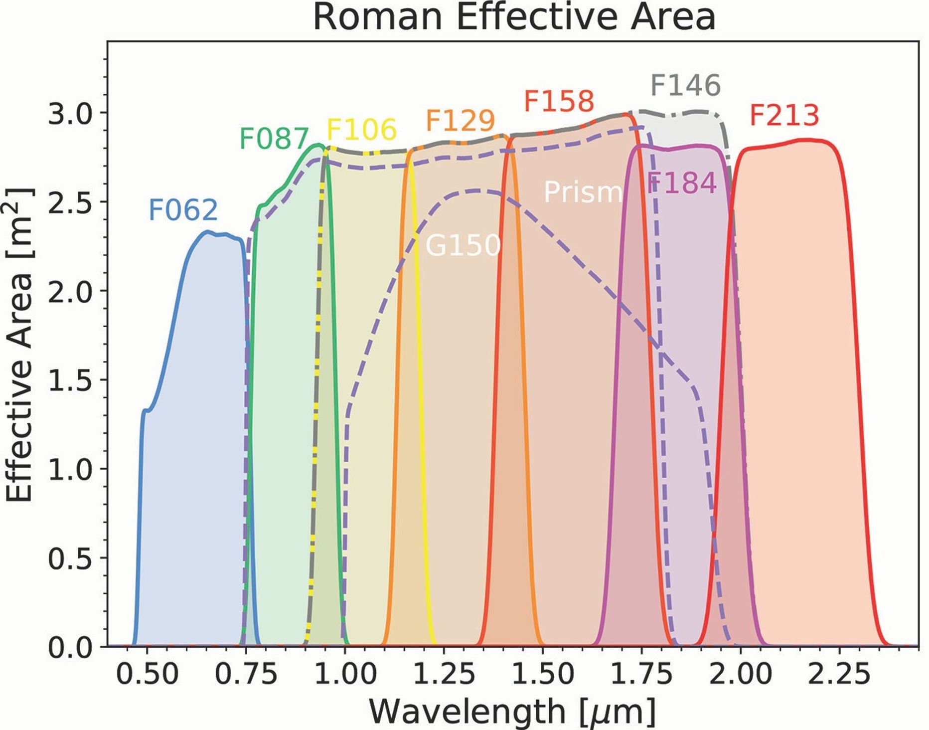
Filters
WFI carries 8 science filters with overlapping band passes spanning 0.48 – 2.3 microns. The filters are located at the telescope exit pupil. They are housed in the element wheel and are rotated into the instrument light path for multiwavelength imaging.
Filter Point Spread Functions
This update is based on the post-CDR optical design. The wavefront error model includes design residuals and Monte Carlo estimates of surface figure errors and alignment tolerances.
Point spread functions (PSFs) for the Nancy Grace Roman Space Telescope have been created using
STPSF (formerly WebbPSF version 1.0), a Python-based package. This tool takes into account properties of the telescope and the instruments, including detector pixel scale, rotations, filter profiles, and point source spectra. These are not full optical models, simply a tool that transforms the optical path difference maps, into the resulting Roman PSFs.
The website linked above provides instructions on how to install STPSF, how to run it via the Python API, in addition to providing Roman specific examples.
Imaging PSFs were calculated at the center of each SCA and also around the periphery of the focal plane; located at the center of a pixel and at the corner of a pixel.
Filter Design Parameters
| Corner PSF | Center PSF | ||||||||
|---|---|---|---|---|---|---|---|---|---|
| Element name | Min (μm) | Max (μm) | Center (μm) | Width (μm) | PSF FWHM (arcsec) * | n eff pixel | Peak Flux | n eff pixel | peak flux |
| F062 | 0.48 | 0.76 | 0.620 | 0.280 | 0.058 | 7.35 | 0.20341 | 3.80 | 0.49536 |
| F087 | 0.76 | 0.977 | 0.869 | 0.217 | 0.073 | 9.35 | 0.16517 | 4.04 | 0.4838 |
| F106 | 0.927 | 1.192 | 1.060 | 0.265 | 0.087 | 10.96 | 0.15060 | 4.83 | 0.44004 |
| F129 | 1.131 | 1.454 | 1.293 | 0.323 | 0.106 | 11.79 | 0.14863 | 6.63 | 0.36874 |
| F158 | 1.380 | 1.774 | 1.577 | 0.394 | 0.128 | 12.63 | 0.14343 | 9.65 | 0.29081 |
| F184 | 1.683 | 2.000 | 1.842 | 0.317 | 0.146 | 17.15 | 0.11953 | 15.52 | 0.21361 |
| F213 | 1.95 | 2.30 | 2.125 | 0.35 | 0.169 | 20.38 | 0.10831 | 20.14 | 0.17052 |
| F146 | 0.927 | 2.000 | 1.464 | 1.030 | 0.105 | 12.18 | 0.14521 | 7.37 | 0.34546 |
Access machine-readable version.
Download all the PSF FWHM (arcsec) * [.ZIP]
*Note: PSF FWHM in arcseconds simulated for a detector near the center of the WFI FOV using an input spectrum for a K0V type star. Please click on the FWHM value for each filter to view the simulated PSF.
The above table provides representative PSF FWHM values for a detector (SCA 1) near the center of the WFI FOV. Wavelength distribution is that of a K0V star, sampled over each filter bandpass. N Eff Pix is number of effective pixels (aka noise pixels) under the PSF (1/sum of squares of pixel values). Fluxes normalized at telescope exit pupil. Images are ~7 arcsec square and typically contain 97%-99% of the incident flux. Two cases are provided: at the corner of 4 pixels, and at the center of a pixel.
FWHM (arcsec) of PSF is computed from 8-times oversampled PSF. Gaussian pointing jitter with FWHM = 8 mas is included. The number of noise pixels and maximum flux per pixel are computed on native detector pixels.
Roman Effective Area Curves
(updated March 2024)
The Roman effective area has been updated to reflect recalibration of the sensor ship assembly (SCA) quantum efficiency, and preliminary updates to the filter, prism, and grism bandpasses. The tables have also been broken out by SCA to illustrate the small differences in QE and the shift in filter bandpasses with field angle. Download the Filter Effective Area tables [.ZIP]
The tables are in ECSV format, which can be read via astropy.io.ascii.read() and any text editor.
The plot below illustrates both these effects by comparing the effective area for SCAs 1 and 9 for filter F158.
Access machine-readable version.
Download all the PSF FWHM (arcsec) * [.ZIP]
*Note: PSF FWHM in arcseconds simulated for a detector near the center of the WFI FOV using an input spectrum for a K0V type star. Please click on the FWHM value for each filter to view the simulated PSF.
The above table provides representative PSF FWHM values for a detector (SCA 1) near the center of the WFI FOV. Wavelength distribution is that of a K0V star, sampled over each filter bandpass. N Eff Pix is the number of effective pixels (aka noise pixels) under the PSF (1/sum of squares of pixel values). Fluxes normalized at telescope exit pupil. Images are ~7 arcsec square and typically contain 97%-99% of the incident flux. Two cases are provided: at the corner of 4 pixels, and at the center of a pixel.
FWHM (arcsec) of PSF is computed from 8-times oversampled PSF. Gaussian pointing jitter with FWHM = 8 mas is included. The number of noise pixels and maximum flux per pixel are computed on native detector pixels.
Roman Effective Area Curves
(updated March 2024)
The Roman effective area has been updated to reflect recalibration of the sensor ship assembly (SCA) quantum efficiency, and preliminary updates to the filter, prism, and grism bandpasses. The tables have also been broken out by SCA to illustrate the small differences in QE and the shift in filter bandpasses with field angle. Download the Filter Effective Area tables [.ZIP]
The tables are in ECSV format, which can be read via astropy.io.ascii.read() and any text editor.

The bandpass shifts given here are representative models; these will be updated once the full set of data from the wide-field instrument thermal vacuum test has been obtained and analyzed.
Measured Field-Dependent Filter Edge Wavelengths (Updated March 2026)
The table provides field-dependent red and blue edge wavelengths based on coating witness measurements. In the table, the "edge" wavelengths refer to the wavelengths where filter transmission crosses through 50%. Errors in the effective index estimate are typically +/- 0.07 and yield 0.06% fractional tolerance in the edge wavelength variation across the field. Additionally, the indices and coating thickness of the flight optics may differ from the witnesses. A future update will provide edges and field dependence measured from the flight coatings at operational temperature. The table provides convenient estimates of field dependence. Filter witness measurements and relation to flight optics are described in Switzer et al. (2025).
SCA | F062 blue edge (nm) | F062 red edge (nm) | F087 blue edge (nm) | F087 red edge (nm) | F106 blue edge (nm) | F106 red edge (nm) | F129 blue edge (nm) | F129 red edge (nm) | W146 blue edge (nm) | W146 red edge (nm) | F158 blue edge (nm) | F158 red edge (nm) | F184 blue edge (nm) | F184 red edge (nm) | F213 blue edge (nm) | F213 red edge (nm) |
|---|---|---|---|---|---|---|---|---|---|---|---|---|---|---|---|---|
| 1 | 482.39 | 761.8 | 763.0 | 983.55 | 935.26 | 1201.3 | 1129.44 | 1455.04 | 927.28 | 2003.07 | 1386.97 | 1785.89 | 1685.4 | 2007.22 | 1966.02 | 2315.24 |
| 2 | 482.22 | 761.46 | 762.66 | 983.13 | 934.86 | 1200.8 | 1129.0 | 1454.45 | 926.92 | 2002.19 | 1386.43 | 1785.2 | 1684.73 | 2006.42 | 1965.22 | 2314.31 |
| 3 | 481.44 | 759.97 | 761.19 | 981.31 | 933.1 | 1198.59 | 1127.09 | 1451.84 | 925.31 | 1998.33 | 1384.02 | 1782.18 | 1681.77 | 2002.9 | 1961.69 | 2310.2 |
| 4 | 481.69 | 760.45 | 761.67 | 981.9 | 933.67 | 1199.3 | 1127.71 | 1452.68 | 925.83 | 1999.58 | 1384.8 | 1783.16 | 1682.73 | 2004.04 | 1962.83 | 2311.53 |
| 5 | 481.61 | 760.3 | 761.52 | 981.71 | 933.49 | 1199.08 | 1127.52 | 1452.42 | 925.67 | 1999.19 | 1384.56 | 1782.85 | 1682.43 | 2003.69 | 1962.47 | 2311.12 |
| 6 | 480.98 | 759.1 | 760.33 | 980.24 | 932.07 | 1197.3 | 1125.98 | 1450.32 | 924.37 | 1996.08 | 1382.62 | 1780.42 | 1680.05 | 2000.85 | 1959.63 | 2307.81 |
| 7 | 480.24 | 757.69 | 758.94 | 978.5 | 930.4 | 1195.21 | 1124.17 | 1447.84 | 922.85 | 1992.41 | 1380.34 | 1777.55 | 1677.25 | 1997.51 | 1956.29 | 2303.91 |
| 8 | 480.49 | 758.16 | 759.4 | 979.07 | 930.95 | 1195.9 | 1124.76 | 1448.66 | 923.35 | 1993.62 | 1381.09 | 1778.49 | 1678.17 | 1998.61 | 1957.39 | 2305.2 |
| 9 | 480.22 | 757.64 | 758.89 | 978.45 | 930.35 | 1195.14 | 1124.1 | 1447.76 | 922.8 | 1992.29 | 1380.27 | 1777.45 | 1677.15 | 1997.4 | 1956.17 | 2303.78 |
| 10 | 482.41 | 761.84 | 763.04 | 983.6 | 935.31 | 1201.36 | 1129.49 | 1455.11 | 927.32 | 2003.17 | 1387.03 | 1785.97 | 1685.47 | 2007.31 | 1966.11 | 2315.35 |
| 11 | 482.24 | 761.51 | 762.72 | 983.2 | 934.92 | 1200.88 | 1129.07 | 1454.55 | 926.97 | 2002.34 | 1386.51 | 1785.31 | 1684.83 | 2006.55 | 1965.35 | 2314.46 |
| 12 | 481.47 | 760.03 | 761.26 | 981.38 | 933.17 | 1198.68 | 1127.17 | 1451.95 | 925.38 | 1998.5 | 1384.13 | 1782.31 | 1681.9 | 2003.05 | 1961.84 | 2310.38 |
| 13 | 481.8 | 760.67 | 761.88 | 982.16 | 933.93 | 1199.63 | 1127.99 | 1453.07 | 926.06 | 2000.15 | 1385.15 | 1783.6 | 1683.16 | 2004.56 | 1963.35 | 2312.13 |
| 14 | 481.72 | 760.52 | 761.73 | 981.98 | 933.74 | 1199.4 | 1127.79 | 1452.8 | 925.9 | 1999.75 | 1384.9 | 1783.29 | 1682.85 | 2004.19 | 1962.98 | 2311.71 |
| 15 | 481.08 | 759.29 | 760.52 | 980.47 | 932.3 | 1197.58 | 1126.22 | 1450.65 | 924.58 | 1996.57 | 1382.93 | 1780.8 | 1680.42 | 2001.3 | 1960.08 | 2308.33 |
| 16 | 480.39 | 757.97 | 759.21 | 978.84 | 930.73 | 1195.62 | 1124.52 | 1448.33 | 923.15 | 1993.13 | 1380.79 | 1778.11 | 1677.8 | 1998.17 | 1956.94 | 2304.68 |
| 17 | 480.64 | 758.46 | 759.7 | 979.45 | 931.31 | 1196.35 | 1125.15 | 1449.19 | 923.68 | 1994.4 | 1381.58 | 1779.11 | 1678.77 | 1999.33 | 1958.1 | 2306.03 |
| 18 | 480.37 | 757.93 | 759.17 | 978.79 | 930.68 | 1195.56 | 1124.47 | 1448.26 | 923.1 | 1993.03 | 1380.73 | 1778.03 | 1677.72 | 1998.07 | 1956.85 | 2304.57 |
Access machine-readable version
Imaging Sensitivity
Imaging Sensitivity Overview
(Updated June 3, 2024)
The table below gives the 5-sigma AB magnitude limiting sensitivity, for twice the minimum zodiacal light background (roughly equivalent to that obtained at an ecliptic latitude of 25 degrees at a Solar elongation of 90 degrees), for 57 second and one-hour integrations, for point sources and a compact galaxy with half-light radius of 0.3 arcseconds.
S/N was computed for photometric apertures of radius 2 pixels for point sources and 6 pixels for the galaxies.
| Filter | F062 | F087 | F106 | F129 | F158 | F184 | F213 | F146 |
|---|---|---|---|---|---|---|---|---|
| Wavelength (microns) | 0.48-0.76 | 0.76-0.98 | 0.93-1.19 | 1.13-1.45 | 1.38-1.77 | 1.68-2.00 | 1.95-2.30 | 0.93-2.00 |
| 1 hr, Point | 27.97 | 27.63 | 27.60 | 27.60 | 27.52 | 26.95 | 25.64 | 28.01 |
| 1 hr, r50=0.3” | 26.70 | 26.38 | 26.37 | 26.37 | 26.37 | 25.95 | 24.71 | 26.84 |
| 57s, Point | 24.77 | 24.46 | 24.46 | 24.43 | 24.36 | 23.72 | 23.14 | 25.37 |
| 57s, r50=0.3” | 23.53 | 23.23 | 23.26 | 23.24 | 23.24 | 22.76 | 22.23 | 24.22 |
Access machine-readable version
Scalings for other deep cases: The flux density limit for other deep integrations, between about ten minutes and tens of hours, can be estimated from the 1 hour depths using a flux ∝ t-1/2 scaling. For integrations below about 10 minutes, this scaling becomes over-optimistic by > 30% due to read noise and overheads. Limits for a half-light radius of 0.2” are slightly closer to the 0.3” case than the point source case. For more extended sources, the limiting flux density fν,lim for fixed SNR and integration time should be scaled from the 0.3” case approximately as fν,lim∝r50 or ΔABlim=2.5 log(0.3"/r50). Reducing the assumed zodiacal background from 2x to 1.44x minimum improves deep imaging flux limits by about 0.15 mag for the F062 through F158 filters, 0.08 mag for F184 and F146, and negligibly for F213.
Fast/Wide Limit: The final two lines in the table give magnitude limits achieved at 5σ in 55 seconds (with a single exposure). At this integration time, Roman can cover approximately 8 contiguous square degrees per hour in one spectral element, and slew-and-settle overheads slightly exceed integration time. There is little point considering faster survey speeds, because sensitivity drops rapidly for modest increases in survey speed at yet shorter integrations.
Zodiacal Light and Thermal Background
(Updated June 3, 2024)
The tables below provides the count rate per pixel at minimum Zodiacal light in each filter and the estimated thermal background. For observations at high galactic latitudes, the Zodi intensity is typically ~1.5x the minimum. For observation into the galactic bulge, the Zodi intensity is typically 2.5-7x the minimum.
| Count rate per pixel at minimum Zodiacal Light | |||||||
|---|---|---|---|---|---|---|---|
| F062 | F087 | F106 | F129 | F158 | F184 | F213 | F146 |
| 0.25 | 0.251 | 0.277 | 0.267 | 0.244 | 0.141 | 0.118 | 0.781 |
Access machine-readable version.
| Internal thermal backgrounds (count rate per pixel) | |||||||
|---|---|---|---|---|---|---|---|
| F062 | F087 | F106 | F129 | F158 | F184 | F213 | F146 |
| 0.003 | 0.003 | 0.003 | 0.003 | 0.048 | 0.155 | 4.38 | 1.03 |
Access machine-readable version.
Imaging Sensitivity Calculator
(Note: data files have *not* yet been updated)
On this page you will find tools designed to help you, the user, calculate the exposure time required for a given source at a given signal to noise, or vice versa.
We have provided a Jupyter notebook which walks through each step of the calculation, and a python script that will open a GUI in which you can input your objects information.
To run both scripts you will need to download the accompanying data files.
Both the notebook and the GUI require the user to specify the filter, zodiacal light contribution, type of source, fitting method, and signal to noise. In this notebook we will be doing exposure time calculations for point sources, and extended sources with half-light radii of 0.2 arcsec or 0.3 arcsec.
- Filters: F062, F087, F106, F129, F158, F184, F146, F213
- Zodiacal light contributions (multiples of the minimum): 1.2, 1.4, 2.0, 3.5
- Source: point sources, objects with a half-light radius (HLR) = 0.2", objects with a HLR = 0.3"
- Fit with a PSF (Point source only)
- Fit with a 2 pixel circular aperture (Point source & HLR = 0.2")
- Fit with a 3 pixel circular aperture
- Fit with a 4 pixel circular aperture
- Fit with a 5 pixel circular aperture (HLR = 0.3" only)
- Fit with a 6 pixel circular aperture (HLR = 0.2" & 0.3" only)
- S/N: 5, 10, 15, 20, 50
The exposure times used within these calculations are quantized in multiples of 3 readout frames, with the number of visits/dithers being 1.
An example of using the Jupyter notebook is provided here.
Spectroscopy
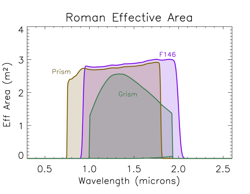
WFI carries 2 dispersive elements for slitless, multi-object spectroscopy. The grism band pass spans 1.0 – 1.93 microns and has a resolution of ~600. The prism band pass spans 0.75 – 1.80 microns and has a resolution of ~100. The dispersing elements are housed in the element wheel and are rotated into the instrument light path for slitless spectroscopy across the WFI FOV.
Grism and Prism parameters
| Element name | Min (μm) | Max (μm) | Center (μm) | Width (μm) | R |
|---|---|---|---|---|---|
| G150 | 1.0 | 1.93 | 1.465 | 0.930 | 461 * wavelength [microns] |
| P127 | 0.75 | 1.80 | 1.275 | 1.05 | 80-180 (2pix) |
Access machine-readable version.
Grism and Prism Effective Area Curves
The effective area as a function of wavelength for the filters, grism, and prism are available in tabular form here.
Grism and Prism zodiacal light
The table below provides the count rate per pixel at minimum zodiacal light for the grism and prism. For observations at high galactic latitudes, the Zodi intensity is typically ~1.5x the minimum. For observation into the galactic bulge the Zodi intensity is typically 2.5-7x the minimum.
| Count rate per pixel at minimum zodiacal light | |
|---|---|
| Grism | Prism |
| 0.65 | 0.95 |
Access machine-readable version.
Grism Spectroscopy Sensitivity
(updated June 11, 2024)
The Roman WFI slitless grism has a spectral range of 1.00-1.93 microns and a dispersion of about 1.1 nm/pixel, essentially independent of wavelength, yielding a 2-pixel resolving power of R = λ / δλ = 460 λ / μm for a point source. Table gives 5-sigma detection limits for a one-hour exposure time with zodiacal light background at twice the minimum intensity. This is representative of an ecliptic latitude of 25 degrees and 90 degrees ecliptic longitude relative to the Sun (the middle of the object visibility window). Typical HLWAS backgrounds are ~30% lower.
For emission lines, the values are integrated line fluxes in units of 10-17 ergs/cm2/sec.
For continua, the values are the AB magnitude at which S/N=5 per pixel.
The values are averages over all 18 detectors; typical variations from one detector to another are 0.05 to 0.1 mag for the continuum cases and ~10% for the emission line limits.
| 5σ limits for Roman WFI grism in 1 hour on source, 2x minimum zodiacal background.Emission line limits are in units of 10-17 erg cm-2 s-1, and continuum limits are in AB mags for 1 pixel | ||||||||||
|---|---|---|---|---|---|---|---|---|---|---|
| Wavelength (microns) | 1.05 | 1.1 | 1.2 | 1.3 | 1.4 | 1.5 | 1.6 | 1.7 | 1.8 | 1.9 |
| fline,17, r50=0; 1 hour | 5.9 | 4.7 | 3.6 | 3.2 | 3.0 | 3.1 | 3.3 | 3.7 | 3.4 | 4.7 |
| mAB, r50=0; 1 hour | 21.3 | 21.5 | 21.6 | 21.6 | 21.5 | 21.3 | 21.2 | 21.0 | 20.8 | 20.4 |
| fline,17, r50=0.3"; 1 hour | 16.1 | 12.9 | 9.8 | 8.7 | 7.6 | 8.1 | 8.4 | 8.9 | 8.5 | 11.7 |
| mAB (2 pix), r50=0.3",1 hour | 20.5 | 20.6 | 20.8 | 20.7 | 20.6 | 20.5 | 20.3 | 20.2 | 20.0 | 19.6 |
Access machine-readable version.
Sensitivities for other integration times (between a few minutes and tens of hours) and zodiacal backgrounds can be scaled from the above using f lim∝t-1/2 b1/2, where t is integration time and b the zodiacal background level. Because this is slitless spectroscopy, the scaling of sensitivity with size for r∝r50 > 0.3" differs between line and continuum sensitivity, with limiting behaviors of flne ∝r50, and fcont ∝r501/2.
Prism Spectroscopy Sensitivity
(updated June 11, 2024)
The Roman WFI slitless prism has a spectral range of 0.75-1.80 microns and a resolution that is strongly wavelength dependent, with 80 < λ / δλ < 180. The highest resolution is at the blue end of the prism wavelength coverage. In addition to its lower dispersion, the prism has higher throughput than the grism, making it more sensitive to continuum. The table below has AB magnitude at which S/N=5 per pixel (not per 2 pixels as earlier), at zodiacal light at twice minimum. This is representative of an ecliptic latitude of 25 degrees and 90 degrees ecliptic latitude relative to the Sun (middle of the object visibility window). Typical HLWAS backgrounds are ~30% lower.
These are averages over all 18 detectors; typical variations from one detector to another are 0.05 to 0.1 mag.
| 5σ limits for Roman WFI prism, 2x minimum zodiacal background | ||||||
|---|---|---|---|---|---|---|
| Wavelength | 0.80 | 1.00 | 1.20 | 1.40 | 1.60 | 1.75 |
| Δλ (for 1 pixel, in nm) | 2.2 | 4.4 | 5.6 | 8.2 | 9.3 | 9.1 |
| mAB(1 pix), r50=0; 1 hour | 22.6 | 23.2 | 23.4 | 23.4 | 23.3 | 23.3 |
| mAB(1 pix), r50=0.3"; 1 hour | 22.0 | 22.6 | 22.8 | 22.8 | 22.8 | 22.7 |
| mAB(1 pix), r50=0; 62 sec | 19.9 | 20.4 | 20.6 | 20.7 | 20.6 | 20.5 |
| mAB(1 pix), r50=0.3"; 62 sec | 19.3 | 19.9 | 20.1 | 20.1 | 20.1 | 20.0 |
Access machine-readable version.
The same scalings that apply to grism spectroscopy can be used to scale other deep prism sensitivities from the 1-hour case.
Grism and Prism dispersion (updated March 2026)
Roman/WFI grism dispersion at the field center based on measurements from WFI TVAC2 combined with the Roman optical model. The field dependence of the grism dispersion is described in Bray et al. (2024). Users interested in a full model of the grism dispersion should contact Eric Switzer.

Access machine-readable version.
Roman/WFI prism dispersion at the field center based on measurements from WFI TVAC2 combined with the Roman optical model. Analysis is ongoing to model the prism dispersion in the regime > 1600 nm and dispersions at those wavelengths in this file are not fully calibrated. Users interested in wavelengths >1600 nm, the field dependence of the prism dispersion, and/or a full model of the prism dispersion should contact Eric Switzer and refer to Bray et al. (2024). The prism design is described in Eegholm et al. (2025).

Access machine-readable version.
Grism Edge Wavelengths (updated March 2026)
The table provides field-dependent red and blue edge wavelengths based on coating witness measurements. In the table, the “edge" wavelengths refer to the wavelengths where filter transmission crosses through 50%. Errors in the effective index estimate are typically +/- 0.07 and yield 0.06% fractional tolerance in the edge wavelength variation across the field. Additionally, the indices and coating thickness of the flight optics may differ from the witnesses. A future update will provide edges and field dependence measured from the flight coatings at operational temperature. The table provides convenient estimates of field dependence. Filter witness measurements and relation to flight optics are described in Switzer et al. (2025).
| SCA | Grism Blue Edge (nm) | Grism Red Edge (nm) |
|---|---|---|
| 1 | 996.82 | 1923.14 |
| 2 | 996.72 | 1922.92 |
| 3 | 995.61 | 1920.66 |
| 4 | 995.79 | 1921.02 |
| 5 | 995.92 | 1921.29 |
| 6 | 994.98 | 1919.35 |
| 7 | 993.45 | 1916.22 |
| 8 | 994.04 | 1917.43 |
| 9 | 993.71 | 1916.75 |
| 10 | 996.75 | 1922.98 |
| 11 | 996.63 | 1922.74 |
| 12 | 995.5 | 1920.43 |
| 13 | 995.41 | 1920.25 |
| 14 | 995.55 | 1920.52 |
| 15 | 994.65 | 1918.67 |
| 16 | 992.96 | 1915.22 |
| 17 | 993.51 | 1916.35 |
| 18 | 993.22 | 1915.75 |
Prism Edge Wavelengths (updated March 2026)
The table provides field-dependent red and blue edge wavelengths based on coating witness measurements. Errors in the effective index estimate are typically +/- 0.07 and yield 0.06% fractional tolerance in the edge wavelength variation across the field. Additionally, the indices and coating thickness of the flight optics may differ from the witnesses. A future update will provide edges and field dependence measured from the flight coatings at operational temperature. The table provides convenient estimates of field dependence. Filter witness measurements and relation to flight optics are described in Switzer et al. (2025).
Additionally, the prism red edge has field dependence defined by coatings on both sides of the optic, which is not fully captured by the table and is the focus of ongoing work. The blue edge should be used as a primary anchor.
| SCA | Prism Blue Edge (nm) | Prism Red Edge (nm) |
|---|---|---|
| 1 | 759.87 | 1823.21 |
| 2 | 758.63 | 1819.87 |
| 3 | 756.58 | 1814.36 |
| 4 | 759.15 | 1821.27 |
| 5 | 757.99 | 1818.17 |
| 6 | 756.17 | 1813.27 |
| 7 | 757.24 | 1816.15 |
| 8 | 756.8 | 1814.97 |
| 9 | 755.5 | 1811.45 |
| 10 | 759.8 | 1823.02 |
| 11 | 758.54 | 1819.64 |
| 12 | 756.5 | 1814.14 |
| 13 | 758.86 | 1820.51 |
| 14 | 757.72 | 1817.44 |
| 15 | 755.91 | 1812.56 |
| 16 | 756.82 | 1815.01 |
| 17 | 756.39 | 1813.84 |
| 18 | 755.07 | 1810.3 |
Access machine-readable version.
Focal Plane System
Updated January 2025
Roman/WFI Focal Plane System (FPS) Sensor Chip Assembly (SCA) Performance Measurements
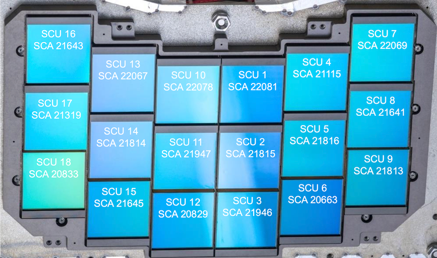
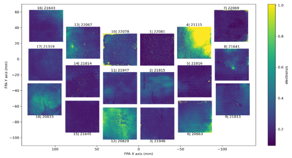
These measurements were performed on either individual flight SCAs in the NASA Goddard Detector Characterization Lab (DCL) at a temperature of 95 K or on the full flight focal plane during WFI Thermal Vaccuum Test #2 (TVAC2) in the nominal operation (NomOp) test plateau at a temperature of 89.5 K. The test parameters for each performance measurement are noted in the descriptions. In these data tables individual detectors are described by either their Sensor Control Unit (SCU) number, which defines their position in the focal plane array as an integer 1 through 18, or their SCA serial number, which is a 5 digit integer that defines each individual detector. Please refer to the SCU to SCA mapping table and labeled diagram of the flight focal plane array for reference.
Roman/WFI SCU to SCA mapping
Sensor control unit (SCU) number to sensor ship assembly (SCA) serial number mapping.
| SCU# | SCA |
|---|---|
| 1 | 22081 |
| 2 | 21815 |
| 3 | 21946 |
| 4 | 21115 |
| 5 | 21816 |
| 6 | 20663 |
| 7 | 22069 |
| 8 | 21641 |
| 9 | 21813 |
| 10 | 22078 |
| 11 | 21947 |
| 12 | 20829 |
| 13 | 22067 |
| 14 | 21814 |
| 15 | 21645 |
| 16 | 21643 |
| 17 | 21319 |
| 18 | 20833 |
Access machine-readable table.
WFI CDS Noise Summary
Roman/WFI TVAC2 Nominal Operation (at 89.5 K) correlated double sampling (CDS) noise measurements (mean and medians) for each SCA.
| SCU | SCA | CDS Noise - Median (e-) | CDS Noise - Mean (e-) |
|---|---|---|---|
| 1 | 22081 | 17.49 | 17.92 |
| 2 | 21815 | 14.2 | 14.43 |
| 3 | 21946 | 14.7 | 15.34 |
| 4 | 21115 | 15.76 | 16.33 |
| 5 | 21816 | 13.64 | 15.93 |
| 6 | 20663 | 13.65 | 14.06 |
| 7 | 22069 | 13.21 | 13.63 |
| 8 | 21641 | 12.49 | 12.72 |
| 9 | 21813 | 12.39 | 12.57 |
| 10 | 22078 | 15.75 | 16.17 |
| 11 | 21947 | 13.94 | 14.25 |
| 12 | 20829 | 13.73 | 13.88 |
| 13 | 22067 | 16.17 | 16.56 |
| 14 | 21814 | 13.46 | 13.68 |
| 15 | 21645 | 13.46 | 13.72 |
| 16 | 21643 | 13.49 | 13.74 |
| 17 | 21319 | 12.64 | 12.82 |
| 18 | 20833 | 12.42 | 12.59 |
| All Detectors (MPA) | - | 13.81 | 14.46 |
Access machine-readable version.
WFI Total Noise
Roman/WFI TVAC2 Nominal Operation (89.5 K) total noise measurements (means, medians, and percentage of pixels passing the total noise requirement) for each SCA.
Roman/WFI total noise measured for each Sensor Control Unit (SCU). Total noise data were acquired from WFI TVAC2 measurements of 100 total exposures, each with a ~170-second integration time, consisting of 55 non-destructive reads and 0 skip frames. Specifically, 50 exposures were taken with the Guide Window (GW) at the bottom left of each sensor chip assembly, and 50 with the GW at the top right. Data analysis included top and column reference pixel correction (using a Savitzky-Golay filter), slope calculation of digital number per unit time per pixel using all frames, and total noise calculation per pixel as the standard deviation of the slopes multipliedby the total exposure time (~170-seconds). A global conversion gain was then applied to convert the results to electrons.
| SCU | SCA | Total Noise - median (e-) | Total Noise - mean (e-) | Percentage Passing Requirement (%) |
|---|---|---|---|---|
| 1 | 22081 | 6.67 | 7.52 | 98.86 |
| 2 | 21815 | 5.6 | 6.02 | 99.59 |
| 3 | 21946 | 5.76 | 6.19 | 99.45 |
| 4 | 21115 | 5.9 | 6.5 | 99.53 |
| 5 | 21816 | 5.76 | 6.38 | 99.48 |
| 6 | 20663 | 5.42 | 5.97 | 99.48 |
| 7 | 22069 | 5.38 | 5.99 | 99.37 |
| 8 | 21641 | 5.13 | 5.54 | 99.58 |
| 9 | 21813 | 5.33 | 5.7 | 99.62 |
| 10 | 22078 | 6.1 | 6.85 | 98.69 |
| 11 | 21947 | 5.86 | 6.25 | 99.52 |
| 12 | 20829 | 5.51 | 5.9 | 99.64 |
| 13 | 22067 | 6.25 | 6.85 | 99.08 |
| 14 | 21814 | 5.41 | 5.85 | 99.59 |
| 15 | 21645 | 5.31 | 5.75 | 99.58 |
| 16 | 21643 | 5.37 | 5.8 | 99.56 |
| 17 | 21319 | 5.14 | 5.54 | 99.62 |
| 18 | 20833 | 5.17 | 5.6 | 99.56 |
| All Detectors (MPA) | - | 5.58 | 6.12 | 99.43 |
Access machine-readable version.
WFI Dark Current Summary
Roman/WFI TVAC2 Nominal Operation (89.5 K) dark current measurements (means, medians, and percentage of pixels passing the dark current requirement) for each SCA.
NOTE: These measurements are representative of the instrument internal thermal background rather than the true dark current floor of the detectors.
| SCU | SCA | Dark Current - Median (e-/s) | Dark Current - Mean (e-/s) | Percentage Passing Requirement (%) |
|---|---|---|---|---|
| 1 | 22081 | 0.019 | 0.049 | 99.63 |
| 2 | 21815 | 0.018 | 0.023 | 99.95 |
| 3 | 21946 | 0.019 | 0.026 | 99.95 |
| 4 | 21115 | 0.018 | 0.038 | 99.85 |
| 5 | 21816 | 0.030 | 0.042 | 99.84 |
| 6 | 20663 | 0.016 | 0.028 | 99.83 |
| 7 | 22069 | 0.027 | 0.044 | 99.78 |
| 8 | 21641 | 0.016 | 0.022 | 99.94 |
| 9 | 21813 | 0.017 | 0.019 | 99.97 |
| 10 | 22078 | 0.012 | 0.033 | 99.74 |
| 11 | 21947 | 0.029 | 0.035 | 99.94 |
| 12 | 20829 | 0.020 | 0.022 | 99.97 |
| 13 | 22067 | 0.013 | 0.023 | 99.89 |
| 14 | 21814 | 0.018 | 0.024 | 99.94 |
| 15 | 21645 | 0.016 | 0.020 | 99.95 |
| 16 | 21643 | 0.017 | 0.023 | 99.94 |
| 17 | 21319 | 0.013 | 0.016 | 99.98 |
| 18 | 20833 | 0.015 | 0.018 | 99.96 |
| All Detectors (MPA) | - | 0.018 | 0.028 | 99.89 |
Access machine-readable table.
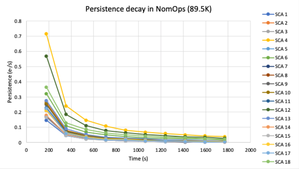
WFI Persistence Summary
Roman/WFI TVAC2 Nominal Operation (89.5 K) persistence measurements as a function of time for each SCA. The persistence decay was measured using 10 regularly spaced darks spanning a total time of 1770 secs (~30 min) following exposures of 56 frames each where the detectors were exposed to ~900 e-/s flat field illumination, for a total of ~159 ke- of charge accumulation.
| Time (sec) | SCU 1 | SCU 2 | SCU 3 | SCU 4 | SCU 5 | SCU 6 | SCU 7 | SCU 8 | SCU 9 | SCU 10 | SCU 11 | SCU 12 | SCU 13 | SCU 14 | SCU 15 | SCU 16 | SCU 17 | SCU 18 | |
|---|---|---|---|---|---|---|---|---|---|---|---|---|---|---|---|---|---|---|---|
| 177.072 | 0.146235 | 0.26914 | 0.208909 | 0.715303 | 0.166129 | 0.321581 | 0.170376 | 0.221845 | 0.249611 | 0.257818 | 0.229222 | 0.568741 | 0.276093 | 0.178377 | 0.165413 | 0.211329 | 0.224006 | 0.36455 | |
| 354.144 | 0.044841 | 0.080633 | 0.059426 | 0.241064 | 0.0463 | 0.10913 | 0.049536 | 0.064649 | 0.07482 | 0.07682 | 0.069049 | 0.184668 | 0.090751 | 0.051928 | 0.045952 | 0.064078 | 0.059692 | 0.1285 | |
| 531.216 | 0.023507 | 0.045668 | 0.03181 | 0.145959 | 0.022286 | 0.068685 | 0.027701 | 0.039115 | 0.040834 | 0.048665 | 0.035978 | 0.111288 | 0.052541 | 0.024169 | 0.022562 | 0.037347 | 0.031434 | 0.086216 | |
| 708.288 | 0.016631 | 0.031565 | 0.021515 | 0.107611 | 0.015596 | 0.051404 | 0.017754 | 0.025009 | 0.028098 | 0.030286 | 0.025927 | 0.078931 | 0.035089 | 0.018905 | 0.014848 | 0.022405 | 0.017657 | 0.063135 | |
| 885.36 | 0.009396 | 0.023053 | 0.01332 | 0.080936 | 0.011316 | 0.037807 | 0.01423 | 0.017882 | 0.020321 | 0.024215 | 0.018094 | 0.064139 | 0.028408 | 0.011699 | 0.010885 | 0.021261 | 0.017525 | 0.050066 | |
| 1062.432 | 0.00984 | 0.016082 | 0.008898 | 0.06767 | 0.009273 | 0.031754 | 0.011129 | 0.014292 | 0.014158 | 0.020825 | 0.014174 | 0.051971 | 0.024368 | 0.008673 | 0.008435 | 0.013684 | 0.009487 | 0.042402 | |
| 1239.504 | 0.00582 | 0.014848 | 0.008599 | 0.058597 | 0.005292 | 0.026527 | 0.008026 | 0.011552 | 0.0108 | 0.015552 | 0.010313 | 0.044002 | 0.016293 | 0.007313 | 0.006979 | 0.011272 | 0.010245 | 0.034529 | |
| 1416.576 | 0.006392 | 0.01378 | 0.003147 | 0.050338 | 0.006203 | 0.024131 | 0.001806 | 0.008925 | 0.008713 | 0.014692 | 0.007939 | 0.03745 | 0.016612 | 0.004375 | 0.004713 | 0.009337 | 0.006833 | 0.032375 | |
| 1593.648 | 0.003686 | 0.008991 | 0.002982 | 0.043606 | 0.002584 | 0.022399 | 0.009896 | 0.008839 | 0.007807 | 0.011118 | 0.006973 | 0.03421 | 0.013128 | 0.005231 | 0.006142 | 0.006756 | 0.003648 | 0.025551 | |
| 1770.72 | 0.003665 | 0.006856 | 0.006162 | 0.038372 | 0.002049 | 0.017933 | 0.005152 | 0.004193 | 0.006178 | 0.011545 | 0.005599 | 0.027749 | 0.009889 | 0.002241 | 0.003875 | 0.006386 | 0.00417 | 0.021669 |
Access machine-readable table.
Roman/WFI TVAC2 Nominal Operation (89.5 K) exponential decay fits to persistence measurements as a function of time for each SCA. The median persistence (e-/s over the dark current) was fit to an exponential function with this form: a*e-bx+d*e-ex+c, where x is the time in the decay curve and a, b, c, d, and e are fit coefficients provided in this file.
| SCU | a | b | c | d | e |
|---|---|---|---|---|---|
| 1 | 0.0630975242491005 | 0.00223961641358588 | 0.0025742933824052 | 0.746862190043635 | 0.011286859153504 |
| 2 | 0.113667333605889 | 0.00208090919789521 | 0.00529851744032986 | 1.63240804741764 | 0.012290801561742 |
| 3 | 0.127692713448231 | 0.0028105284087841 | 0.002995637210518 | 1.79386542406018 | 0.0148971770132734 |
| 4 | 0.317245856240149 | 0.0020385294263819 | 0.0313180347386418 | 3.84258893619047 | 0.0119526816052686 |
| 5 | 0.0399074220360969 | 0.0010724842266948 | -0.00399342219621827 | 0.818575758396395 | 0.0100903092011291 |
| 6 | 0.171722202455368 | 0.00229210782641212 | 0.0165894251978556 | 2.23092490376614 | 0.0138939156373566 |
| 7 | 0.0903847550202783 | 0.00265170572847035 | 0.00464743580396528 | 1.24816990075988 | 0.0137579427881678 |
| 8 | 0.120784603994506 | 0.00245260186948826 | 0.00484601419324385 | 2.08785922359341 | 0.0153109677593873 |
| 9 | 0.116569528810883 | 0.00226588275130876 | 0.00414036289741852 | 1.52550646007652 | 0.0124780793195191 |
| 10 | 0.168943431158506 | 0.00288223884036085 | 0.0108454245616368 | 4.10029537346811 | 0.0188524408598509 |
| 11 | 0.0819994803715525 | 0.00184109607970523 | 0.00230678758276112 | 1.17683690959174 | 0.0110023229183419 |
| 12 | 0.219784999387394 | 0.00185549271970522 | 0.0213015004890999 | 3.04482947488278 | 0.0116175577250163 |
| 13 | 0.097603576989658 | 0.00163228812268123 | 0.00539309058027533 | 1.26391264016757 | 0.0104807084599246 |
| 14 | 0.0493188990667302 | 0.00151680485718246 | -0.000556202364831174 | 0.852045139438995 | 0.0101491228354148 |
| 15 | 0.0554350616724502 | 0.00227001770532573 | 0.00342068217961765 | 0.880160085914408 | 0.0110268563640265 |
| 16 | 0.0847549639343177 | 0.00193252760814128 | 0.00346770668447426 | 1.20674682246829 | 0.0118640541303733 |
| 17 | 0.062650881955819 | 0.00163596315647808 | 0.000329354246793926 | 1.27435292812059 | 0.011155677866177 |
| 18 | 0.175415985545229 | 0.00182390269280901 | 0.0163324746934558 | 2.39421963631299 | 0.0134505500033584 |
Access machine-readable table.
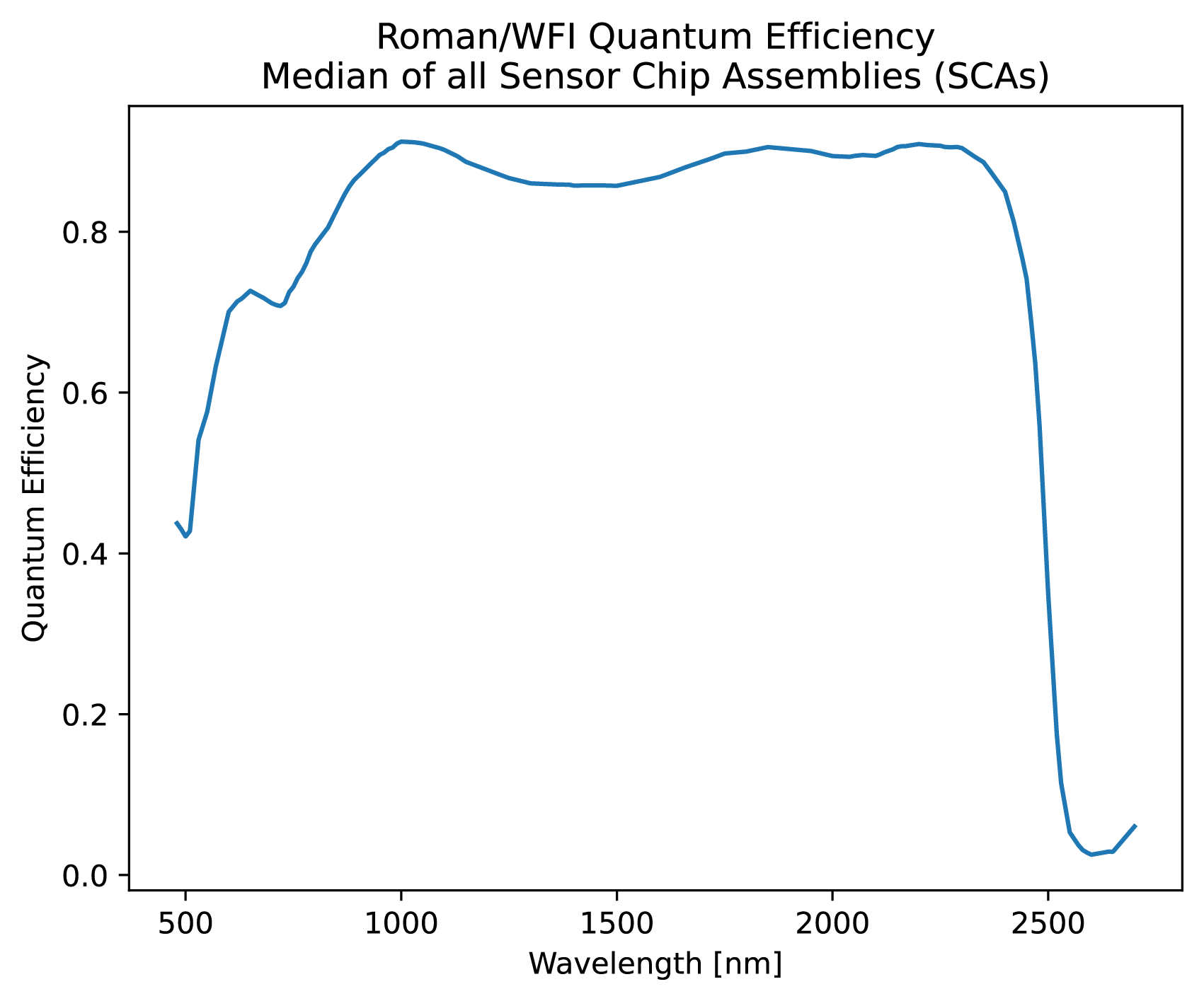
WFI Quantum Efficiency
Roman/WFI Detector Characterization Lab measurements of the median quantum efficiency (QE) versus wavelength (linearly interpolated) for each SCA.
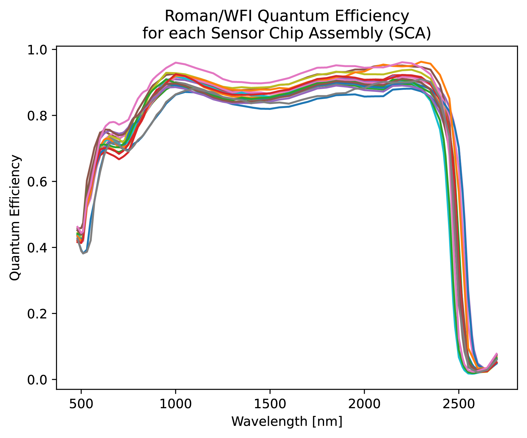
For the measured quantum efficiency of each SCA versus wavelength (measured every 10 nm), please see this machine-readable table.
Short and Long Wavelength Quantum Efficiencies
| Wavelength Range | Mean Quantum Efficiency | Median Quantum Efficiency |
|---|---|---|
| wavelengths < 900 nm | 0.694 | 0.718 |
| 900 <= wavelengths <= 2200 nm | 0.887 | 0.888 |
The mean and median quantum efficiencies for all WFI SCAs for wavelengths < 900 nm and also 900 <= wavelengths <= 2200 nm.
Short and Long Wavelength Cutoffs
Wavelengths between which the quantum efficiency >=50% for each Sensor Control Unit (SCU).
| SCU | Short (nm) | Long (nm) |
|---|---|---|
| 1 | 560 | 2480 |
| 2 | 530 | 2480 |
| 3 | 530 | 2490 |
| 4 | 530 | 2480 |
| 5 | 530 | 2520 |
| 6 | 520 | 2480 |
| 7 | 530 | 2510 |
| 8 | 530 | 2470 |
| 9 | 530 | 2480 |
| 10 | 530 | 2440 |
| 11 | 530 | 2520 |
| 12 | 530 | 2500 |
| 13 | 520 | 2450 |
| 14 | 530 | 2480 |
| 15 | 530 | 2480 |
| 16 | 520 | 2470 |
| 17 | 530 | 2460 |
| 18 | 570 | 2470 |
| Median | 530 | 2480 |
Access machine-readable table.
WFI Number of Pixels that Meet Requirements
Roman/WFI TVAC2 Nominal Operation (89.5 K) pixel operability statistics. For each SCA this includes the number of pixels deemed inoperable, which do not meet requirements ("bad pixels"), and the percentage of pixels deemed operable that do meet requirements ("good pixels") for each SCA. The performance metrics that can contribute to a pixel being inoperable are dark current, total noise, linearity, persistence, QE, flat field response, gain, and electrical connectivity.
NOTE: SCU/SCA 4/21115 has a significantly lower operable pixel fraction due to an extended region of the detector with persistence that is somewhat larger than the requirement.
| SCU | SCA | Number of Bad Pixels | Percentage Good Pixels (%) |
|---|---|---|---|
| 1 | 22081 | 374528 | 97.76 |
| 2 | 21815 | 107330 | 99.36 |
| 3 | 21946 | 175996 | 98.95 |
| 4 | 21115 | 2548467 | 84.75 |
| 5 | 21816 | 114616 | 99.31 |
| 6 | 20663 | 130840 | 99.22 |
| 7 | 22069 | 236249 | 98.59 |
| 8 | 21641 | 129869 | 99.22 |
| 9 | 21813 | 98921 | 99.41 |
| 10 | 22078 | 258521 | 98.45 |
| 11 | 21947 | 132721 | 99.21 |
| 12 | 20829 | 85538 | 99.49 |
| 13 | 22067 | 315293 | 98.11 |
| 14 | 21814 | 116282 | 99.3 |
| 15 | 21645 | 87095 | 99.48 |
| 16 | 21643 | 93282 | 99.44 |
| 17 | 21319 | 94341 | 99.44 |
| 18 | 20833 | 135371 | 99.19 |
| All Detectors (MPA) | - | - | 98.26 |
Access machine-readable table.
The Roman Wide Field Instrument Relative Calibration System
The Relative Calibration System (RCS) is an optical light source used to calibrate the WFI in flight. The RCS performance has been extensively characterized during TVAC1 & 2. It can flatfield every pixel in the WFI over ~5 orders of magnitude in flux in 6 distinct wavelengths bands; this capability will be the workhorse use case of the RCS on-orbit, used for a slew of calibration programs. The RCS has two primary sub-systems. A "Sphere "(RCSS), which consists of an aluminum exterior shell with 24 LED sources (2 redundant banks of 6 LEDs) that illuminate a Spectralon interior. The LED light illuminating the interior of the sphere is projected onto a fold mirror by a Winston cone optic and reflected to diffusers associated with the back of the Dark element or filter masks to project flat fields onto the focal plane array. The Sphere also hosts photodiodes to independently measure LED flux.
The other RCS subsystem is a redundant set of electronics boxes that provide the commanding and telemetry interface to the RCSS.
The RCS LEDs support the calibration and long term trending of multiple detector properties, including the flux dependent nonlinearity (FDNL; for more details please see Mosby et al. 2020) which primarily impacts the dark energy cosmology science program via observations of type Ia supernovae. FDNL will be constrained in two ways using the RCS:
- The Lamp-on-lamp-off (LOLO) method which compares a sky scene with and without an added flat field pedestal of RCS LED light matched to the observation filter.
- Combinatorial flux addition (CFA) which utilizes combinations of stable fluxes from two LEDs at the same wavelength with no light from a sky scene.
For more information, including hardware schematics, and details on operational modes, please see the Roman User Documentation (RDox) article on the RCS.
LED Bandpass Properties

| Filter | RCS LED Band | RCS LED 200K Measured Center (nm) | RCS LED 200K Measured FWHM (nm) |
|---|---|---|---|
| F062 | 1 | 624 | 618 - 627 |
| F087 | 2 | 853 | 845 - 858 |
| F106 | 3 | 1039 | 1021 - 1050 |
| F129 | 4 | 1270 | 1241 - 1293 |
| F158 | 5 | 1481 | 1448 - 1516 |
| F184 | 6 | 1670 | 1622 - 1706 |
Access machine-readable version.
Version History
| Release Number | Date | High-level Release Notes |
|---|---|---|
| v1.4 | March 9, 2026 | Prism+grism dispersions; filter, prism, and grism band edges; Relative Calibration System LEDP info |
| v1.3 | August 13, 2025 | Add version numbering language and fix jitter. |
| v1.2 | June 30, 2025 | Added WFI Technical Overview page |
| v1.1 | January 29, 2025 | Added WFI FPS information and measurements from TVAC2 |
| v1.0 | August 28, 2024 | Initial release of Roman Technical Information |
Please note: these release notes are at a very high level. For all of the details and changes for each release, please visit our Roman Technical Data Repository release page.